Mathematics#
In the following, a brief overview with respect to the inverse problems that can be described when using probeye should be outlined. This requires to define the statistical models (the data generating processes) that can be build from a given deterministic simulation model, as it is assumed to be the case when using this package.
Let us assume that  ,
,  denotes the observed data (observations) of some process that depends on a set of controllable input data which we summarize as
  ,
,  . In probeye it is assumed, that the observations
  are realizations of a data generating process that can be described by a multivariate normal distribution that depends on the input data
  . If
. If  denotes the corresponding random variable, this can be expressed as
(1)#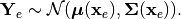
Here,  and
and  refer to the mean vector and the covariance matrix respectively. Next to the previously described observations, we assume that a deterministic forward model
  is available that describes the mean vector
  of the data generating process, that is
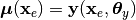
where  ,
,  is the model parameter vector. Since
  is given by the forward model response, the different data generating processes that can be described in probeye only differ in the definition of the covariance matrix
  . The latter depends on the assumed sub-structure of the data generation process. In this context, two general options are supported. A data generation process with an additive or a multiplicative model prediction error. In the first case, Expression (1) is specified to
(2)#
Here,  denotes a Gaussian model for the prediction error, introducing additional latent parameters
  ,
,  , while
 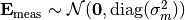 ,
,  describes an independent and identical distributed (i.i.d.) measurement error. The alternative to the additive model prediction error is a multiplicative one. In this case, Expression (1) is specified to
(3)#
where  denotes the unit-mean prediction error while describes the measurement error as defined before. Both data generation processes, Equations (2) and (3), describe a random variable following a multivariate normal distribution as given by (1) where the covariance matrix is given by

Once the mean vector  and the covariance matrix
  are determined, the likelihood of the statistical model can be evaluated via
